Why improve the method from Cabaret & Berrag (2004)?
Source:vignettes/our_improvements.Rmd
our_improvements.RmdThe motivation that led us to propose an improvement over the individual method proposed by the authors is that we identified the two pitfalls mentioned in the previous paragraph, i.e. the arbitrary pair-matching and requirement of an even sample-size.
Hereafter, we demonstrate the issue from the paper’s own toy example.
EPG values import
library(FECR)

set.seed(42)

# Generate random EPG values, in the simple case of equal sample size
T1 <- c(450,1250,1700,900,2550,500,750,850,500)
T1.mean <- mean(T1)
T2 <- c(50,0,0,0,50,450,400,0,0)
T2.mean <- mean(T2)
C1 <- c(750,600,500,700,1000,700,300,1250,1050)
C1.mean <- mean(C1)
C2 <- c(540,400,1000,1750,350,600,900,550,450)
C2.mean <- mean(C2)
FECR calculations
As expected, we find FECR values similar to what the authors report:
# Generate random EPG values, in the simple case of equal sample size
FECR(T1.mean,T2.mean,method = "Kochapakdee")            # 90% in the original paper
## [1] 89.94709
FECR(T1,T2,C1,C2,method = "Dash") # 90% in the original paper## Warning in average_if_required(arg.list): a vector of epg has been provided in
## place of a mean. The arithmetic mean of the vector has been used.## [1] 89.47058
FECR(T2 = T2.mean,C2 = C2.mean,method = "Coles") # 86% in the original paper## [1] 85.47401
FECR(T1,T2,method = "Cabaret1",compute.CI = TRUE) # 83%(58-99%) in the original paper## [1] 82.62164
## attr(,"CI")
## lower.2.5% upper.97.5%
## 60.00000 99.34641
FECR(T1,T2,C1,C2,method = "Cabaret2",compute.CI = TRUE) # 84%(51-97%) in the original paper## [1] 84.02088
## attr(,"CI")
## 2.5% 97.5%
## 60.68754 98.28532
FECR(T1,T2,C1,C2,method = "MacIntosh1",compute.CI = TRUE)## [1] 75.37662
## attr(,"CI")
## 2.5% 97.5%
## 63.61780 86.50022Our proposed method leads to a somewhat comparable value, albeit significantly lowered. We explain more on this hereafter.
Demonstration of the pit-falls
The implicit arbitrary pair-matching
The toy-example’s values only lead to the reported FECR when inputted in their specific order. Shuffling this order is enough to change the FECR value:
set.seed(1000)
# shuffling T and C
new.T <- sample(1:length(T1))
new.C <- sample(1:length(C1))

T1.new <- T1[new.T]
T2.new <- T2[new.T]
C1.new <- C1[new.C]
C2.new <- C2[new.C]

# Recalculating FECRs
FECR(T1.new,T2.new,C1.new,C2.new,method = "Cabaret2",compute.CI = TRUE)
## [1] 61.27418
## attr(,"CI")
## 2.5% 97.5%
## 12.75385 98.14815
FECR(T1.new,T2.new,C1.new,C2.new,method = "MacIntosh1",compute.CI = TRUE)## [1] 75.37662
## attr(,"CI")
## 2.5% 97.5%
## 63.23173 85.67652Note that shuffling obviously has not change EPG distribution in T and C groups:
summary(T1)## Min. 1st Qu. Median Mean 3rd Qu. Max.
## 450 500 850 1050 1250 2550
summary(T1.new)## Min. 1st Qu. Median Mean 3rd Qu. Max.
## 450 500 850 1050 1250 2550
summary(C2)## Min. 1st Qu. Median Mean 3rd Qu. Max.
## 350.0 450.0 550.0 726.7 900.0 1750.0
summary(C2.new)## Min. 1st Qu. Median Mean 3rd Qu. Max.
## 350.0 450.0 550.0 726.7 900.0 1750.0And neither have methods based on group-averaged EPG
FECR(T1.new,T2.new,C1.new,C2.new,method = "Dash") # 90% in the original paper## Warning in average_if_required(arg.list): a vector of epg has been provided in
## place of a mean. The arithmetic mean of the vector has been used.## [1] 89.47058
FECR(T2 = T2.new,C2 = C2.new,method = "Coles") # 86% in the original paper## Warning in average_if_required(arg.list): a vector of epg has been provided in
## place of a mean. The arithmetic mean of the vector has been used.## [1] 85.47401More precisely, here is the bootstrapped distribution of the FECR value itself (not its confidence interval), across several reshuffling:
library(ggplot2)
library(magrittr)

set.seed(9000)

# replicating the shuffling of T and C
FECR.shuffled <- replicate(
  n = 1000,
  simplify = FALSE,
  expr = {
    # shuffle
    new.T <- sample(1:length(T1))
    new.C <- sample(1:length(C1))

    T1.new <- T1[new.T]
    T2.new <- T2[new.T]
    C1.new <- C1[new.C]
    C2.new <- C2[new.C]

    #FECR calculations
    data.frame(
      method = c("Cabaret2","MacIntosh1"),
      FECR = c(
        FECR(T1.new,T2.new,C1.new,C2.new,method = "Cabaret2",compute.CI = FALSE),
        FECR(T1.new,T2.new,C1.new,C2.new,method = "MacIntosh1",compute.CI = FALSE)
      )
    )
  }
) %>%
  do.call(rbind,.)
FECR.shuffled %>%
  ggplot(aes(x = FECR,fill = method))+
  facet_grid(method~.,scales = "free")+
  geom_histogram(binwidth = 2,alpha = 80)+
  guides(fill = "none")+
  scale_x_continuous(limits = c(-1,101))+
  theme_bw()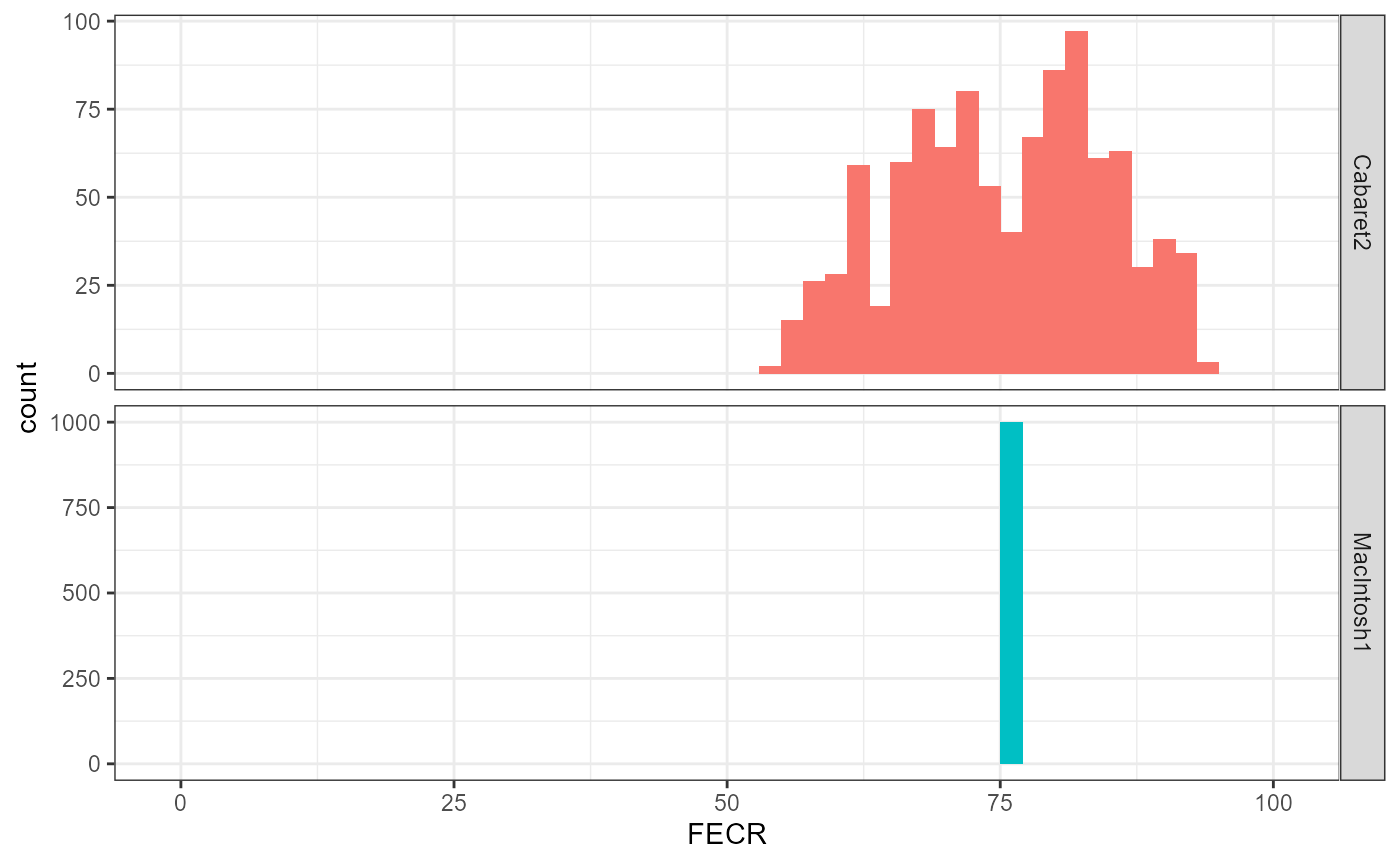
We can see that, depending on how individuals in T and C are paired, Cabaret & Berrag’s method leads to a FECR drawn from a bimodal distribution.
Our method consistently leads to a single FECR value, close to the mean of this distribution:
## [1] 75.37662## [1] 75.30635Uneven sample sizes
Let’s simulate upon this toy example an uneven sample size between the T and C groups by randomly removing 2 individuals from one, e.g. T.
Since the "Cabaret2" method relies on a summation across n individuals in both the T and C groups, this requires subsetting the larger group too by randomly removing 2 individuals. This isn’t a requirement for our method, which will keep using all the individuals from C despite T having 2 individuals less.
set.seed(9999)
# removing 2 individuals from T and C
new.T <- sample(1:length(T1),length(T1) - 2)
new.C <- sample(1:length(C1),length(C1) - 2)

T1.new <- T1[new.T]
T2.new <- T2[new.T]
C1.new <- C1[new.C]
C2.new <- C2[new.C]

# Recalculating FECRs
FECR(T1.new,T2.new,C1.new,C2.new,method = "Cabaret2",compute.CI = TRUE)
## [1] 69.59653
## attr(,"CI")
## 2.5% 97.5%
## 11.15497 99.47090
FECR(T1.new,T2.new,C1,C2,method = "Cabaret2",compute.CI = TRUE)## Error in check_if_valid_parameters(arg.list): Some of T1,T2,C1,C2 are not of the same length.
FECR(T1.new,T2.new,C1,C2,method = "MacIntosh1",compute.CI = TRUE)## [1] 79.13679
## attr(,"CI")
## 2.5% 97.5%
## 64.90151 91.34628Again, if this is replicated many times, FECRs are impacted differently across the two methods:
set.seed(777)

# replicating the shuffling of T and C
FECR.minus.2 <- replicate(
  n = 1000,
  simplify = FALSE,
  expr = {
    # shuffle
    new.T <- sample(1:length(T1),length(T1) - 2)
    new.C <- sample(1:length(C1),length(C1) - 2)

    T1.new <- T1[new.T]
    T2.new <- T2[new.T]
    C1.new <- C1[new.C]
    C2.new <- C2[new.C]

    #FECR calculations
    data.frame(
      method = c("Cabaret2","MacIntosh1"),
      FECR = c(
        FECR(T1.new,T2.new,C1.new,C2.new,method = "Cabaret2",compute.CI = FALSE),
        FECR(T1.new,T2.new,C1,C2,method = "MacIntosh1",compute.CI = FALSE)
      )
    )
  }
) %>%
  do.call(rbind,.)
FECR.minus.2 %>%
  ggplot(aes(x = FECR,fill = method))+
  facet_grid(method~.,scales = "free")+
  geom_histogram(binwidth = 2,alpha = 80)+
  guides(fill = "none")+
  scale_x_continuous(limits = c(-1,101))+
  theme_bw()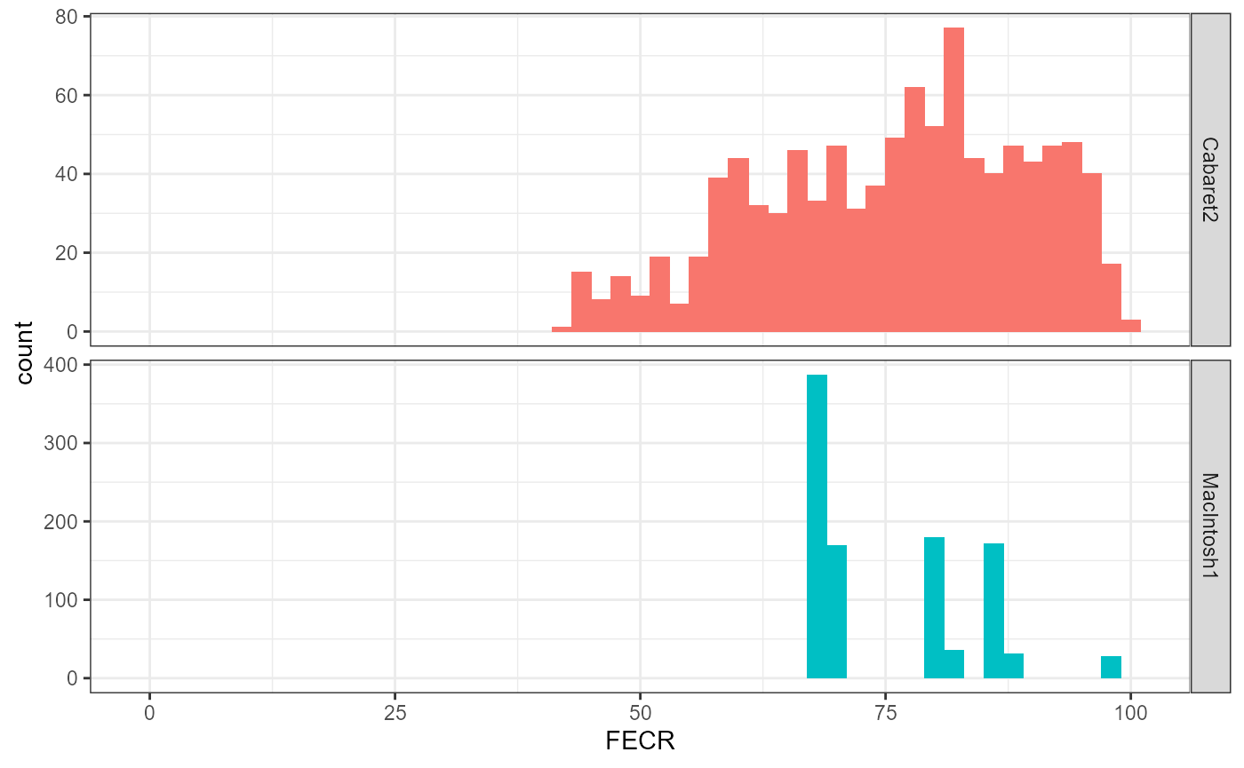
Therefore, on top of using all the data available, our method also leads to more stable FECR values.
What about confidence intervals?
The same processes of reshuffling or removing datapoints can be replicated to calculate the stability of confidence intervals’ boundaries:
set.seed(1234)

# replicating the shuffling of T and C
CI.shuffled <- replicate(
  n = 100,
  simplify = FALSE,
  expr = {
    # shuffle
    new.T <- sample(1:length(T1))
    new.C <- sample(1:length(C1))

    T1.new <- T1[new.T]
    T2.new <- T2[new.T]
    C1.new <- C1[new.C]
    C2.new <- C2[new.C]
    Cab <- FECR(T1.new,T2.new,C1.new,C2.new,method = "Cabaret2",
                          compute.CI = TRUE,pb = FALSE)
    Mac <- FECR(T1.new,T2.new,C1.new,C2.new,method = "MacIntosh1",
                          compute.CI = TRUE,pb = FALSE)

    #FECR calculations
    data.frame(
      method = c("Cabaret2","MacIntosh1"),
      FECR = c(Cab,Mac),
      lower = c(
        attr(Cab,"CI")[1],
        attr(Mac,"CI")[1]
      ),
      upper = c(
        attr(Cab,"CI")[2],
        attr(Mac,"CI")[2]
      )
    )
  }
) %>%
  do.call(rbind,.) %>%
  cbind(rep = factor(rep(1:100,each = 2)),.)
CI.shuffled %>%
  ggplot(aes(method,FECR,colour = method,group = rep))+
  geom_linerange(aes(ymin = lower,ymax = upper),position = position_dodge(.9))+
  geom_point(position = position_dodge(.9))+
  guides(colour = "none")+
  theme_bw()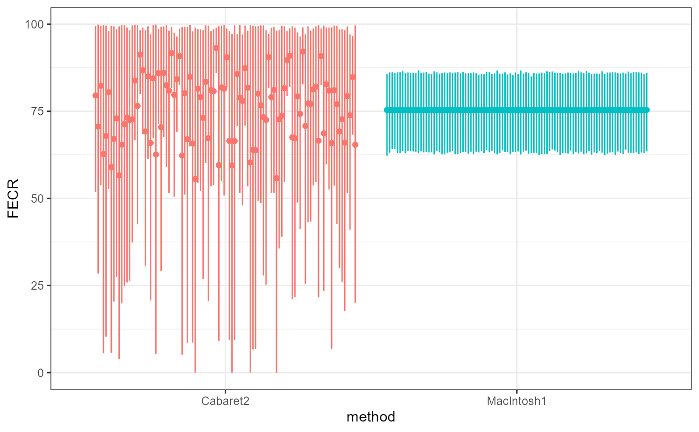
Our proposed method is designed to calculate a FECR value (and its confidence interval) that is unique for a given set of EPG values in T and C groups. The only slight variations observed regarding the boundaries of the confidence interval is attributable to the bootstrap’s own random resampling.
What about multiple values per individual?
None of the methods mentioned so far nor our fix of the Cabaret2 method handle multiple samples per individual. In this FECR package, we propose a non-parametric approach to include individual variability in the FECRs calculation.
Simulating data
Here we simulate values for individuals of groups T and C, with different sample size per individual, group and period.
library(data.table,quietly = TRUE)
library(truncnorm)

set.seed(2001)
# custom simulating function:
sim_epg_data <- function(n,mean,runif.boundaries) {
  lapply(
    1:n,
    function(x) {
      # runif determine a random sample size per individual, and set the epg's sd to twice this
      # value
      runif(1,runif.boundaries[1],runif.boundaries[2]) %>%
        {rtruncnorm(.,mean = mean,sd = . * 2,a = 0)} %>%
        round %>% as.integer
    }
  )
}

# generating the data (generate list-column and unnest them for code brievity)
T1 <- data.table(id = letters[9:18],
                 epg = sim_epg_data(n = 10,mean = 65,c(3,10)))[,.(epg = epg[[1]]),by = id]
T2 <- data.table(id = letters[9:18],
                 epg = sim_epg_data(n = 10,mean = 20,c(6,8)))[,.(epg = epg[[1]]),by = id]
C1 <- data.table(id = letters[1:8],
                 epg = sim_epg_data(n = 8,mean = 70,c(6,12)))[,.(epg = epg[[1]]),by = id]
C2 <- data.table(id = letters[1:8],
                 epg = sim_epg_data(n = 8,mean = 65,c(1,12)))[,.(epg = epg[[1]]),by = id]
Note that ultimately, T1,T2,C1, and C2 now are data.frames (long format) containing column id (referring to the individual identity) and epg (the value per sample). In the future, we will implement ways for the user to specify the column names.
rbind(cbind(group = "Treated",gp = "T1",T1),cbind(group = "Treated",gp = "T2",T2),
      cbind(group = "Control",gp = "C1",C1),cbind(group = "Control",gp = "C2",C2)) %>%
  ggplot(aes(gp,epg,colour = id,fill = id))+
  facet_grid(.~group,scales = "free_x")+
  geom_boxplot(alpha = 0.3)+
  geom_jitter(alpha = .2)+
  guides(colour = "none",fill = "none")+
  xlab("Group per period (before = 1, after = 2)")+
  theme_minimal()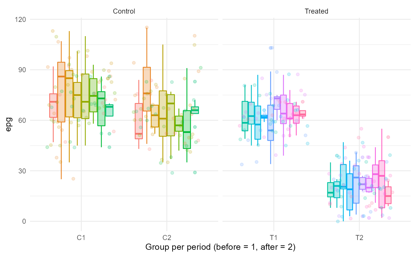
FECR values
With such a dataset, one needs first to average epg values per individual (and possibly by group-period) before using any of the previously mentioned:
rbind(cbind(group = "Treated",gp = "T1",T1),cbind(group = "Treated",gp = "T2",T2),
      cbind(group = "Control",gp = "C1",C1),cbind(group = "Control",gp = "C2",C2)) %>%
  .[,.(epg = mean(epg),l = quantile(epg,.025),u = quantile(epg,.975)),by = .(id,group,gp)] %>%
  ggplot(aes(gp,epg,colour = id,fill = id))+
  facet_grid(.~group,scales = "free_x")+
  geom_line(aes(group = id),alpha = 0.2,colour = "grey50",position = position_dodge(0.2))+
  geom_linerange(aes(ymin = l,ymax = u),position = position_dodge(0.2))+
  geom_point(alpha = .5,position = position_dodge(0.2))+
  guides(colour = "none",fill = "none")+
  xlab("Group per period (before = 1, after = 2)")+
  theme_minimal()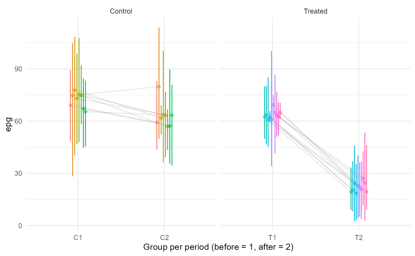
T1.avg <- T1[,.(epg = mean(epg)),by = id]$epg;T2.avg <- T2[,.(epg = mean(epg)),by = id]$epg
C1.avg <- C1[,.(epg = mean(epg)),by = id]$epg;C2.avg <- C2[,.(epg = mean(epg)),by = id]$epg

# returns an error because of the uneven sample size
FECR(T1.avg,T2.avg,C1.avg,C2.avg,method = "Cabaret2",compute.CI = TRUE)
## Error in check_if_valid_parameters(arg.list): Some of T1,T2,C1,C2 are not of the same length.
FECR(T1.avg,T2.avg,C1.avg,C2.avg,method = "MacIntosh1",compute.CI = TRUE)## [1] 60.1642
## attr(,"CI")
## 2.5% 97.5%
## 58.69651 61.46585
# expected FECR given the simulated epg means in the treated group:
1 - (20 / 65) /  (65 / 70)
## [1] 0.6686391We can see that, in this simulation, the FECR value after averaging per individual is lower and less variable than what could be expected by looking at the raw data and inputted mean epgs. Also, note that the confidence interval being so narrow, it does not contain the value 66% obtained through the inputted means.
In comparison, this is how our last method compares:
FECR(T1,T2,C1,C2,boot = 500,method = "MacIntosh2")## [1] 56.00778
## attr(,"CI")
## 2.5% 97.5%
## 34.72859 71.85496
# expected FECR given the simulated epg means in the treated group:
1 - (20 / 65) /  (65 / 70)
## [1] 0.6686391This last method, while returning a mean FECR lower than the one from the previous method, correctly reflects how variable individual epg data are in the dataset, by reprensenting the ditribution of FECR value one could have obtained given the individual variability. Note that this time, the “true” value 66% calculated through the group mean epgs is within the 95% interval.